Types of simulation models – choosing the right approach for a simulation project
 October 30, 2021
 1885 words
 9 minutes to read

Simulation models are not created equal – if you want to build a reliable simulation to propel your business forward, you should understand your problem and what tools are available for its resolution.
No universal models exist that can accurately simulate any business process. Depending on the industry or the nature of the task, the process may change over time or contain many unique unknowns.
The implications are critical: models exist that are great for the team’s specific problem and models that will generate useless results. If the different types of simulation models are understood, then the next steps in the team’s project will be built on a solid footing!
Consequently, today’s goal is to introduce the main types of simulation modeling and appropriate use cases!
Types of simulation models (with examples)
Below are the most notable types of simulation models. To encourage a better grasp of them, each type will be accompanied by simple examples!
Note: Some model types may overlap and those simulation models may be of several types at the same time.
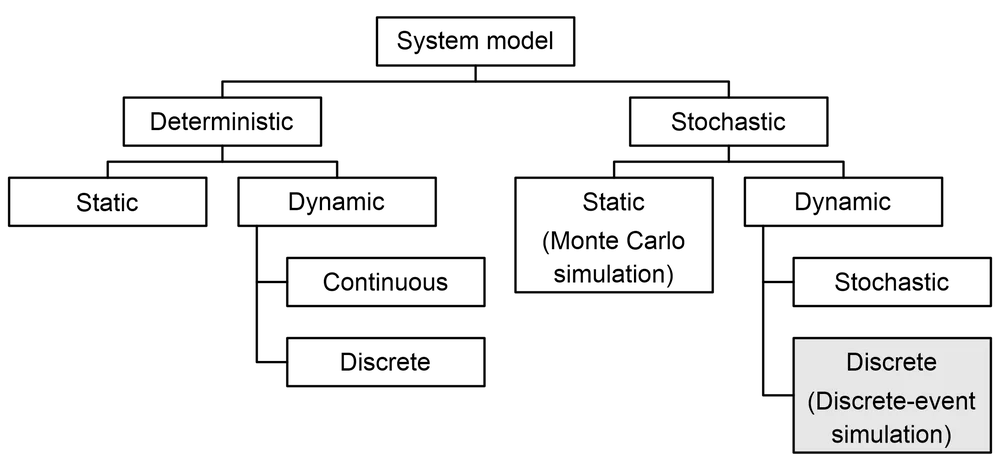
Deterministic vs. stochastic models
Key points – deterministic models are used when the outcomes can be fully predicted, while stochastic models are used when the variables in the process are unknown.
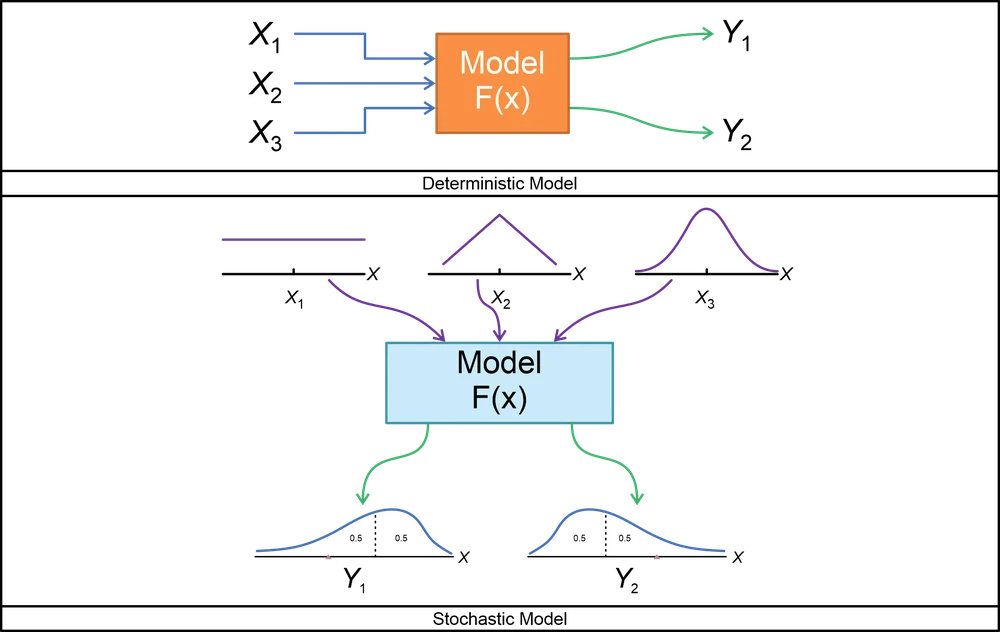
At the highest level, simulation models can be stochastic or deterministic. Here’s how they differ:
- Deterministic models: Applied when dealing with processes whose behavior can be fully predicted from start to end. With a given set of inputs, deterministic models always produce the same outputs. There is no randomness in deterministic models since we know the precise values of all input variables.
- Stochastic models: Applied whenever we cannot accurately estimate input variables – either because we don’t have enough information about the variables or because they fluctuate within a specific range.
As a simple example of a deterministic model, suppose we have a mobile app, and we want to find out how many people will be using it in a month. If we currently have 1,000 users and know that the app will lose 20 users, attract 400 new users, and have 50 returning users within a month, we can easily calculate how many users the app will have in the future.
The calculation would have this quite simple form:
Users in a month = Current users + monthly new users + monthly returning users – monthly leaving users
Or, in our case:
1,000 + 400 + 50 – 20 = 1,430
Unfortunately, in reality, things are frequently much harder than that. Due to various reasons, we may not know for sure how many users we will lose and how many users we will acquire. And that’s where stochastic simulation comes into play!
With stochastic simulation, we can handle uncertainties in the data through probability distributions. Once a suitable probability distribution is chosen for the target process, we can sample data from that distribution, use the data as inputs for our model, and record the model’s outputs. Because we sample values for unknown variables randomly (within a specified distribution), stochastic models produce different results each time we run them.
A more complex example of contrasting and comparing these models can be reviewed for a situation such as pre-positioning disaster response facilities at safe locations (Verma & Gaukler, 2015).
Note: The validity and accuracy of stochastic models depend on how faithfully the selected probability distribution represents the actual process. Therefore, careful preparation and data collection are required for successful simulation.
Static vs. dynamic models
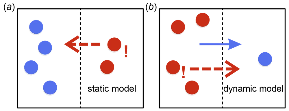
Key points – static models describe a process at one point in time, while dynamic models can represent processes that change and develop over time.
A brief comparison of static and dynamic models is provided below:
- Static models: Applied to simulate processes at a specific instant in time. The outputs of these models only depend on the inputs and internal model variables. Static models produce a snapshot of the process in a specified timeframe.
- Dynamic models: Take into account not only inputs at the current time, but also outputs at previous points in time. Additionally, the output of dynamic models depends on time itself (i.e., variables in dynamic models are denoted as functions of time).
Dynamic models should be used if the target process is known to change over time – perhaps due to seasonality or wear. In contrast, static methods should be used to model systems that stay unchanged as time goes on, or to model systems at a specific time.
Since static models don’t account for how a process evolves, they are unsuitable for non-static processes. For example, if assumptions were made about the sales of a seasonal product based on current market conditions and those assumptions to make predictions were attempted far into the future, then the results would be poor. Our assumptions wouldn’t be able to represent the changed process next week or next month.
Similarly, there’s no point in applying a dynamic model to a process that doesn’t change with time. Dynamic models could still yield valid results when used with static systems, but they would be overkill and require more effort than necessary to simulate a static process. A bit more complex example of contrasting and comparing these models can be reviewed for a situation such as assessing algorithms for predicting drug-drug interactions, (Guest, et al., 2011).
Discrete vs. continuous models

Key points – discrete models are used with systems that change at specific, countable points in time. Continuous models are designed to deal with processes that change continuously.
The main distinctions between discrete and continuous models can be described as follows:
- Discrete models: Applied when the specific instant at which an event occurs, with no changes occurring between events, can be pinpointed. Examples of discrete processes are app downloads, product purchases, or customer arrivals at a bank.
- Continuous models: Applied to processes whose state changes continuously. Examples of continuous processes and phenomena are temperature, speed, or revenue.
In some situations, continuous and discrete models may be used interchangeably, but they may produce results that don’t make sense or are not sufficiently detailed.
For example, if we use a continuous model to simulate software purchases, the model may produce illogical outputs, like 1.5 purchases. Software purchases can be counted, making continuous models unsuitable for their representation (although we could still achieve good results with them).
In contrast, if we use a discrete method to model a continuous process, we may not capture the changes occurring between particular points in time. This may lead to loss of information and thus diminish performance. A more complex example of contrasting and comparing these models can be reviewed for a situation such as tumor-induced angiogenesis, i.e., the formation and development of new blood vessels, (Anderson & Chaplain, 1998).
The Monte Carlo method
Key points – the Monte Carlo method is useful when dealing with random variables in a process. Monte Carlo simulation allows us to determine the likelihood of different outcomes in a system.
The Monte Carlo method is a subtype of stochastic modeling. It relies on the repeated sampling of random inputs from probability distributions. Sampling is carried on until we have enough output data for our needs. The outputs of stochastic models allow us to determine how likely a particular outcome (or a set of outcomes) should occur. This information could later be used for risk analysis or decision-making.
As an example, suppose the estimated annual net profit from a software package that is planned for release to the market is sought. We know that net profit depends on factors like:
- Revenue from software sales.
- Operating expenses.
- Taxes.
These variables are uncertain or random because their values may depend on factors such as:
- The activity levels of the market.
- The costs of developing and maintaining the software.
- Actions of competitors.
We most likely will not accurately calculate net profit because we can’t predict how the market will develop tomorrow. But to obtain at least some basis for calculations, we can observe the process and select a probability distribution(s) to describe it numerically.
After this, to perform a Monte Carlo experiment, we:
- Sample values from our probability distribution.
- Feed these sample values into our model.
- Collect the model’s outputs – the more, the better.
- Observe the interval of outcomes.
Subsequently, we could build a histogram to obtain a graphical view of predicted net profits. If the net profit was discovered to be adequate in the majority of cases, we would decide to proceed with the application. Otherwise, if the loss was more likely, the correct course of action would be to abandon the project or perhaps to reevaluate our steps. A bit more complex example of the Monte Carlo method can be reviewed for a situation such as the meantime to resolution for reported software development bugs (Üsfekes, et al., 2019).
Next steps
Simulation is truly a beautiful discipline – it requires a thoughtful but rigorous approach. But, if used correctly, it can be used to assist development and decision-making in any industry. If the correct model is chosen for the project, the team will be able to:
- Faithfully simulate the target process.
- Quantify uncertainty to be able to make informed decisions.
- Analyze a wide range of outcomes.
Every type of simulation model out there has not been covered in this exercise – many others exist, and the analysis and review of these are encouraged. Remember that awareness of all existing simulation methods is unnecessary! Modern simulation packages provide embedded guidance to help get started regardless of the situation or project. Nonetheless, a general understanding can prove to be very useful! A free course offered through Coursera.org entitled Simulation Models for Decision Making could help the team launch learning about different types of simulation models.
References:
Anderson, A. R., & Chaplain, M. A. J. (1998). Continuous and discrete mathematical models of tumor-induced angiogenesis. Bulletin of Mathematical Biology, 60(5), 857-899.
Guest, E. J., Rowland‐Yeo, K., Rostami‐Hodjegan, A., Tucker, G. T., Houston, J. B., & Galetin, A. (2011). Assessment of algorithms for predicting drug-drug interactions via inhibition mechanisms: comparison of dynamic and static models. British Journal of Clinical Pharmacology, 71(1), 72-87.
Üsfekes, Ç., Tüzün, E., Yılmaz, M., Macit, Y., & Clarke, P. (2019). Auction-based serious game for bug tracking. IET Software, 13(5), 386-392.
Verma, A., & Gaukler, G. M. (2015). Pre-positioning disaster response facilities at safe locations: An evaluation of deterministic and stochastic modeling approaches. Computers & Operations Research, 62, 197-209.