The most important probability distributions for business process simulation
 July 31, 2021
 1932 words
 10 minutes to read
Last Updated: October 16, 2021
10 minutes to read
Last Updated: October 16, 2021

“All models are wrong, but some models are useful.”
– George E. P. Box, renowned statistician
A crucial step in business process simulation is selecting probability distributions to represent simulation inputs. Uncertainty necessitates probability distributions. That is, we never have perfect data and knowledge about the simulated system and its environment. Thus, the need to capture that uncertainty with random variable probability distributions. Once we choose a probability distribution, we may use it to generate random variates in stochastic simulations.
This sounds simple, but before developing a simulation with probabilistic inputs, we need to decide which probability distributions are most appropriate. This article will introduce you to a number of the most important distributions, along with their key properties, for the specific application of business process simulation.
What to know when choosing a probability distribution for simulations
Keep in mind several factors for the use cases, while trying to pinpoint the optimal probability distribution.
1. Choose a probability distribution close to the actual distribution of the data
The chosen probability distribution needs to be sufficiently close to the actual distribution of the data. A solid understanding is necessary for the quantitative and qualitative input data of your simulation. A probability distribution can’t be matched to input data if that input data is not well understood.
2. Choose probability distributions directly related to the use cases
Probability distributions have their distinct use cases. For example, some are intended to model the probability of events with binary outcomes, while others represent the amount of time until the desired event occurs. The nature and role of a simulation input will dictate the type of probability distribution.
3. Distributions require a specific set of parameters for reliable results
Every distribution requires a set of parameters to produce results. Typically, these parameters are statistical measures (such as the mean or standard deviation) describing your data. Before choosing a probability distribution and putting it to use, obtain the values of these parameters.
Important discrete probability distributions for business process simulation
With each of the four probability distributions described below, required parameters are furnished to support an increased understanding of the prerequisites for the probability distributions.
1. Bernoulli distribution
Use this distribution when dealing with single events that only have two possible outcomes.
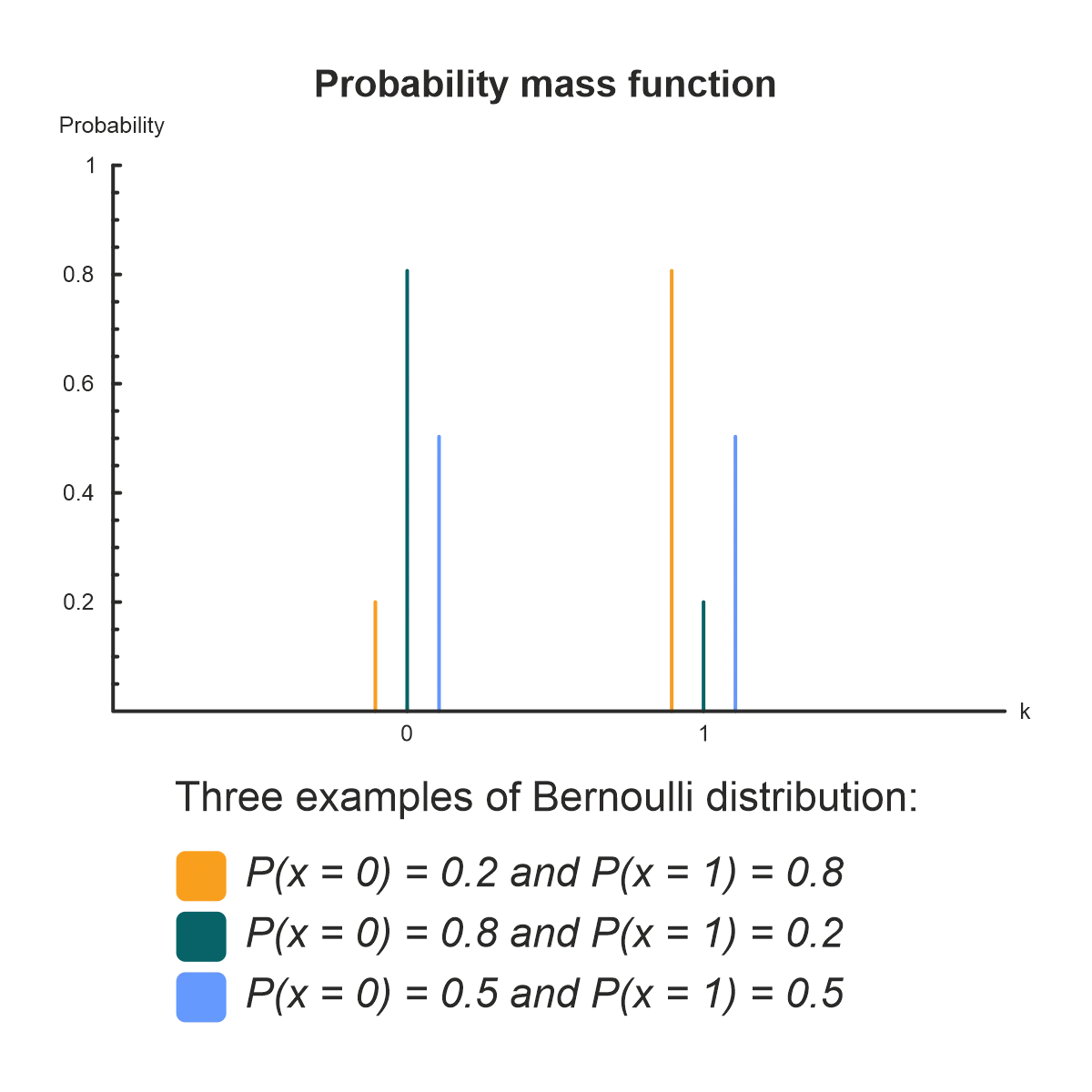
Parameters:
- Probability of success p.
- Probability of failure q = 1 – p.
The Bernoulli distribution represents a single experiment whose outcome has only two possible values. Such experiments are called Bernoulli trials. A simple example of a Bernoulli trial is the toss of a coin where there are two possible outcomes – heads or tails.
The Bernoulli distribution is useful whenever a business process is dealing with a single binary event. For a series of binary events, use the binomial distribution.
2. Binomial distribution
Use this distribution when dealing with a series of experiments that have only two possible outcomes.
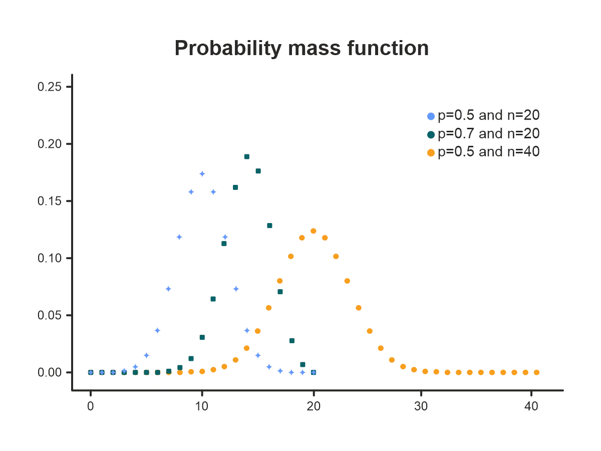
Parameters:
- Number of trials n.
- Probability of success p for each trial.
- Probability of failure q = 1 – p for each trial.
The binomial distribution is the extension of the Bernoulli distribution in that it estimates the probability of a specific number of successes occurring during a series of Bernoulli trials.
This probability distribution may be used in risk management, e.g., when the probability of a product run having a given number of defective pieces or a given number of trucks malfunctioning in a fleet is being assessed.
3. Geometric distribution
Use this distribution when the interest is in the number of undesirable outcomes before a desirable outcome (or the other way around).
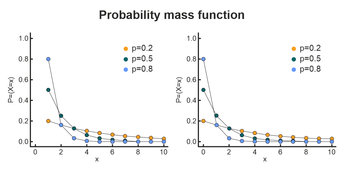
Parameters:
- Probability of success p.
With the geometric distribution, trials have two possible outcomes: yes or no, defective or working, etc. Knowing the probability of success, the likelihood of several failures in succession before the first success can be calculated.
Here, “success” doesn’t necessarily imply a positive or desirable event. The geometric distribution may be turned around, so to speak, and be used to estimate the probability of several desirable results occurring before one undesirable result.
As an example, if the probability with which a machine produces a defective item may be known. The probability of a certain number of working items being produced before one defective item can be computed.
4. Poisson distribution
Use this distribution when the volume times an event will occur in a given time frame must be determined.
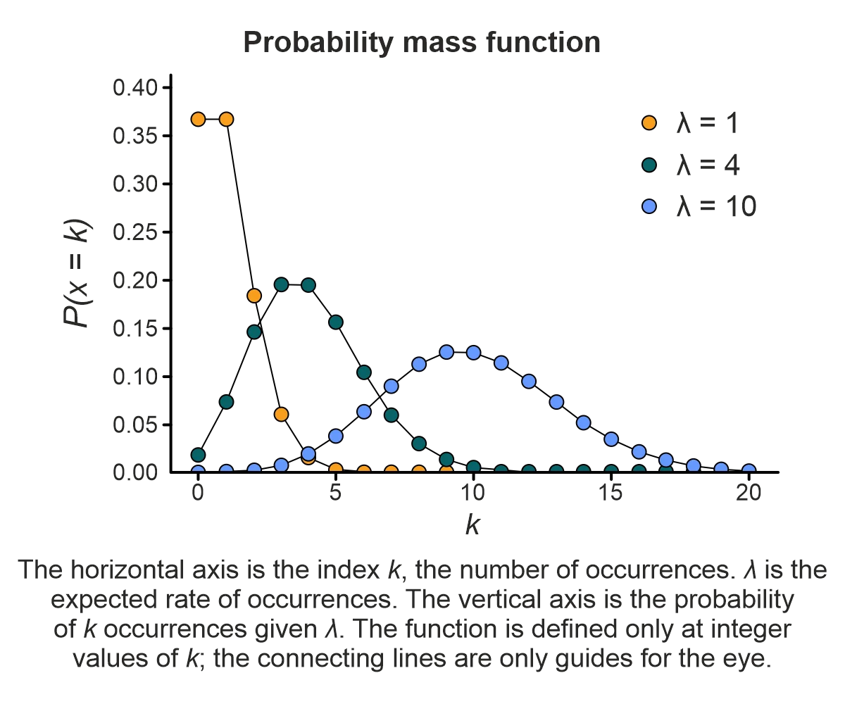
Parameters:
- Average rate of event occurrence λ.
The Poisson distribution represents the probability of a given number of events occurring in a time interval (e.g., one hour, one day, or one week). This distribution assumes that we know the average event occurrence rate λ (Greek letter lambda), that the rate of occurrence is constant, and that the events are independent. That is, the occurrence of one event doesn’t affect the occurrence of the next. A process with these properties is called a Poisson point process.
The Poisson distribution may be used to estimate the likelihood of the:
- Number of calls being made to a customer support center.
- Number of visitors arriving at a store.
- Number of claims made to an insurance company.
Although commonly used with time intervals, the Poisson distribution may also be applied to estimate the probability of events occurring over a distance or area.
Important continuous probability distributions for business process simulation
1. Normal distribution
Use this distribution when the data is symmetric around the mean, with values in proximity to the mean having higher probabilities.
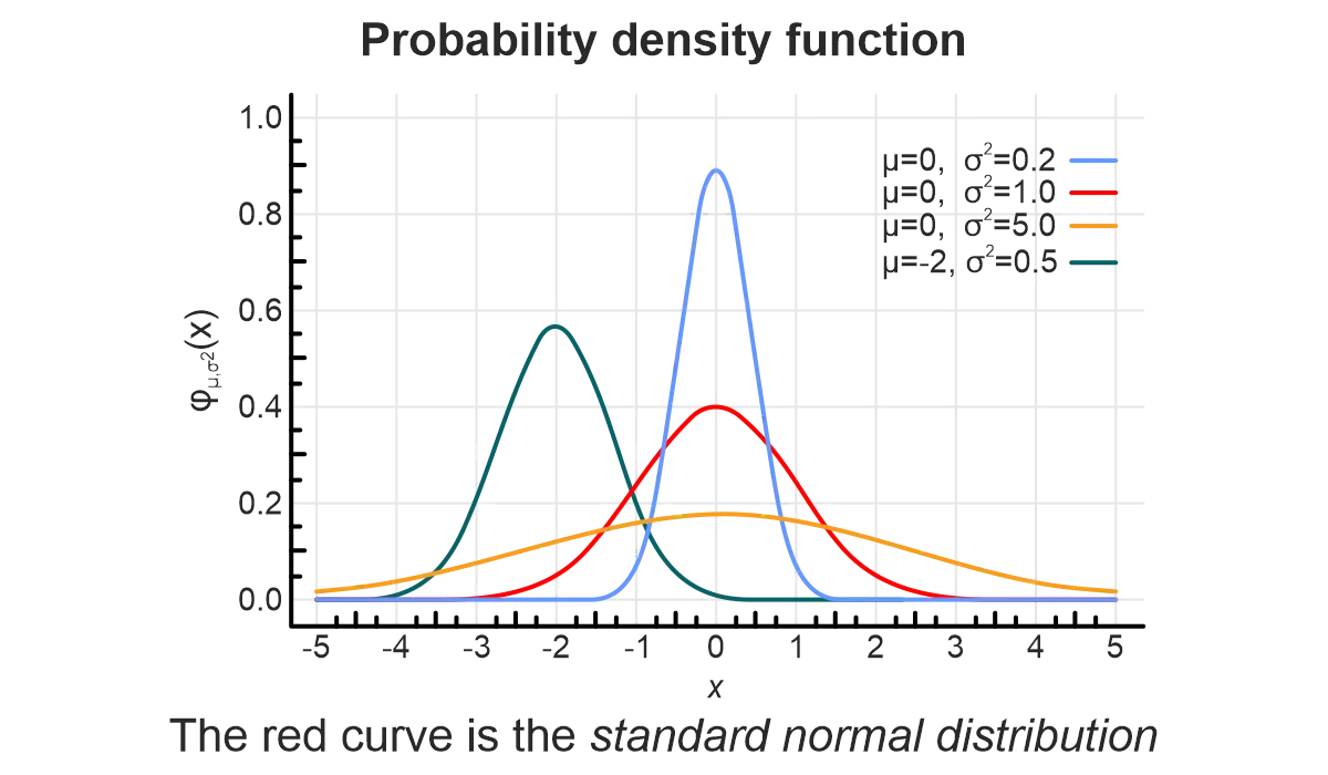
Parameters:
- Mean μ.
- Standard deviation σ or variance σ^2.
The normal distribution (also called Gauss or Gaussian) is the most famous and perhaps the most important continuous probability distribution. The normal distribution can be used to represent many types of real-world events.
An important feature of the normal distribution is that most of its values are symmetrically centered around the mean, thus having higher probabilities. The probability of the values on either side of the mean gradually decreases, giving the distribution curve a characteristic bell shape.
Regardless, values less than one standard deviation away from the mean (in both directions) represent approximately 68.27% of the set, while values two and three standard deviations away account for 95.45% and 99.73%, respectively. This fact is known as the 68-95-99.7 rule.
2. Uniform distribution
Use this distribution when only the lower and upper limits of the input data are known.
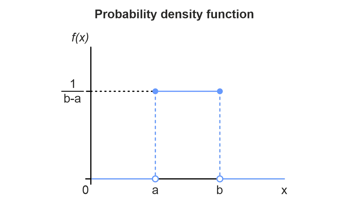
Parameters:
- Lower limit a.
- Upper limit b.
The uniform distribution is commonly used when very little information about the data is available. More specifically, this distribution may be employed when only the lower and upper limits of the input values are known.
The uniform distribution is named “uniform” because the probabilities are equal along the entire distribution curve. Thanks to its simplicity and minimal information requirements, the uniform distribution is sometimes used as the null hypothesis to ascertain the accuracy of mathematical models.
Because probabilities are the same along its distribution curve, the uniform distribution may also be used for sampling data from other distributions. As additional data about a random variable is collected, other distributions may be used for more accurate simulation.
3. Triangular distribution
Use this distribution when the lower and upper limits of the input data are known, and the mode can be estimated.
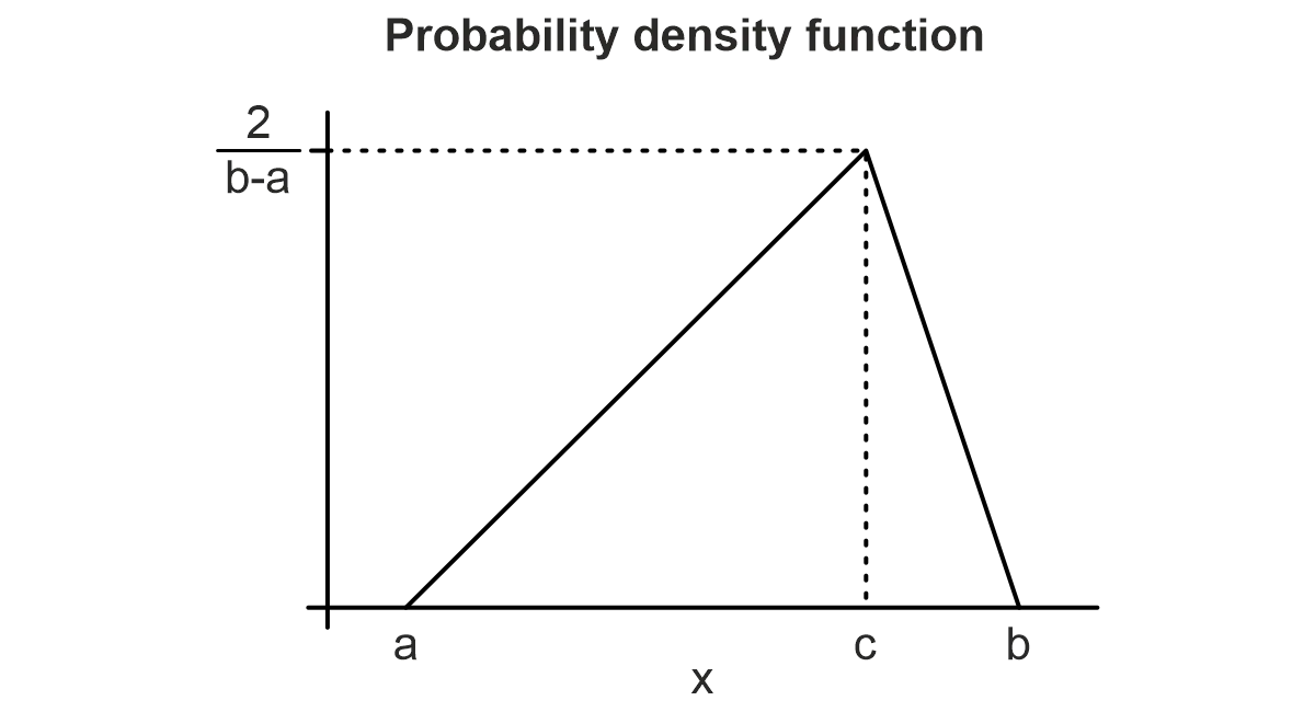
Parameters:
- Lower limit a.
- Upper limit b.
- Mode c.
The triangular distribution is used in situations where limited information about the data is known – similar to the uniform distribution.
However, the triangular distribution also requires the mode of the data points – i.e., the most common value. Additionally, unlike the uniform distribution, values around the mode are more likely, while the probabilities of values closer to the upper and lower bounds are close to zero.
When dealing with a lack of information about the data, accurately calculating the mode may be impossible. Consequently, for an initial simulation, the most likely known outcome as the mode could be used.
4. Exponential distribution
Use this distribution when the time between two events needs to be estimated.
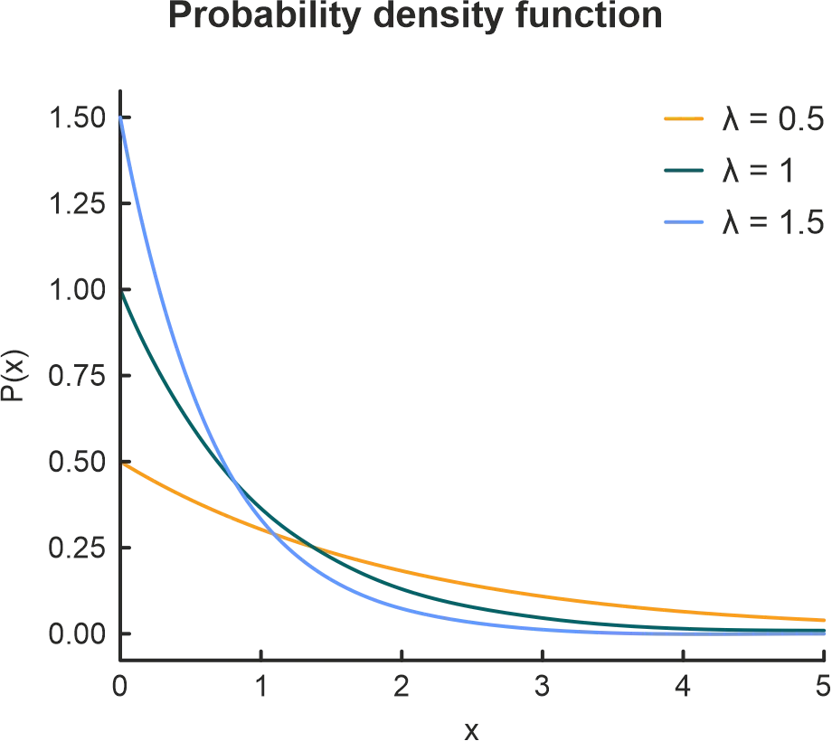
Parameters:
- Average rate of event occurrence λ.
The exponential distribution represents the amount of time between events in a Poisson point process – that is, a process where events occur independently at an average constant rate. This distribution may be viewed as the continuous counterpart of the geometric distribution.
The exponential distribution has a wide range of applications and may be used to estimate the:
- Time until a breakdown in a machine.
- Time between the next order of a product.
- Time until a default on loan payments.
Plotting goodness-of-fit for a probability distribution
Goodness-of-Fit tests are critical to ascertain congruency of the probability distribution to a specific type, the relationship of categorical variables, or the probability distribution source of random samples. A straight, diagonal line means that the simulation contains normally distributed data. The data is not distributed normally if the line is skewed (to the left or right).
Q-Q Plot
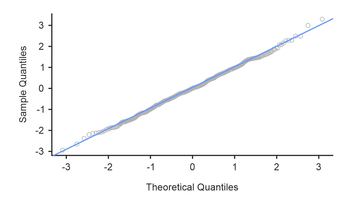
A graphical method to observe the goodness-of-fit for a continuous probability distribution is the Q-Q (Quantile-Quantile) plot. This plot compares the quantiles of sample (empirical) data to the quantiles from a specified probability distribution. When a scatter appears to be a 45º straight line, the sample data will exhibit the continuous uniform distribution under study.
P-P Plot
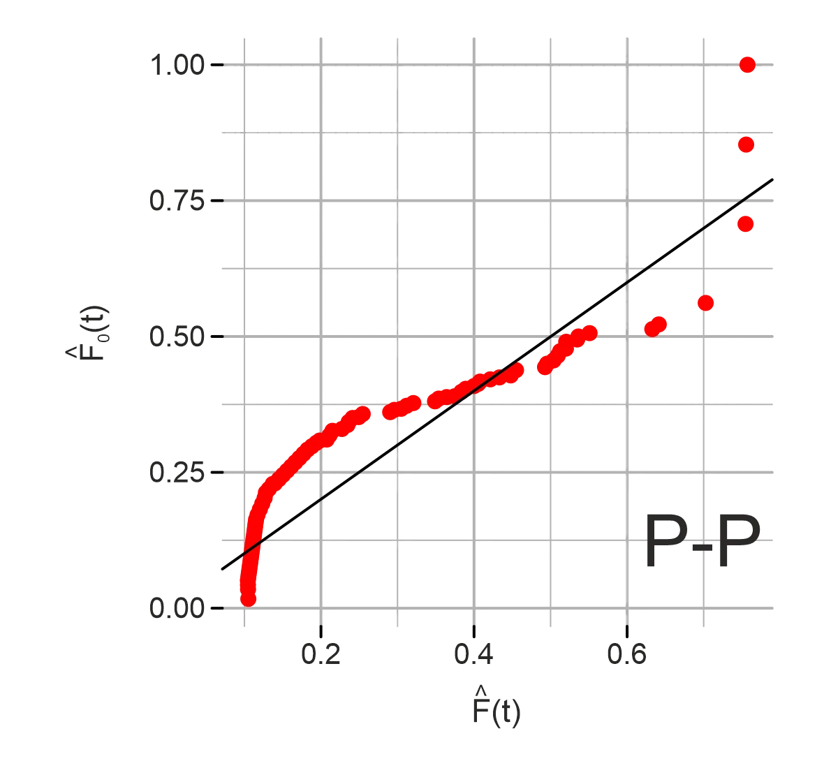
Another graphical method for detecting the goodness-of-fit for both continuous and discrete probability distributions is the P-P (Probability-Probability) plot. This plot compares the cumulative distribution function of the sample (or empirical) data to the cumulative distribution function of a specified probability distribution. Again, the scatter diagram appears as a 45º straight line, where the scales of the x and y-axis are comparable and the angle moves from the lower left-hand side to the upper-right-hand side of the graph.
Next steps
“When a coincidence seems amazing, that’s because the human mind isn’t wired to naturally comprehend probability & statistics.”
– Neil deGrasse Tyson astrophysicist, planetary scientist, author, and science communicator.
One or several variables may play a critical role in the computer simulation model. Often several of the random variables are of the continuous type, while others are discrete. The distributions described above are the most important probability distributions for business process simulation, but there are many more that we haven’t covered, such as continuous probability distributions: lognormal, gamma, beta, and Weibull; and a discrete probability distribution, Pascal.
Remember, no single distribution would suit all use cases – each probability distribution serves its specific purpose. Consequently, a successful simulation is ensured with the definition of the problem being modeled, understanding and properly leveraging the associated data, and the structuring of the correct probability distributions and associated parameters. Consider a free Introduction to Probability and Statistics course from MIT to support your discovery of this topic.
References:
García Carrasco, D. (2017). Goodness-of-fit R package for Right-censored data. (Master’s thesis, Universitat Politècnica de Catalunya). https://upcommons.upc.edu/bitstream/handle/2117/106177/memoria.pdf
Dalpiaz, D. (2017). Applied statistics with R. University of Illinois. Urbana-Champaign, IL. https://daviddalpiaz.github.io/appliedstats/applied_statistics.pdf
Thomopoulos, N. T. (2013). Choosing the Probability Distribution from Data. In Essentials of Monte Carlo Simulation. Springer. (pp. 113-135). https://doi.org/10.1007/978-1-4614-6022-0_10