Introduction to discrete-time simulation
 December 8, 2022
 2983 words
 15 minutes to read

In previous blog posts, we explored various simulation approaches, including continuous and discrete-event simulation (DES). Today, our focus is on discrete-time simulation (DTS) – a simulation technique extremely popular in a wide range of industries, from business to the military.
Choosing the suitable simulation model for a given task is paramount to the success of simulation studies. While some projects can be done with any model, some algorithms are better for specific tasks and entirely unsuitable for others. This also applies to discrete-time simulation – more than many may realize.
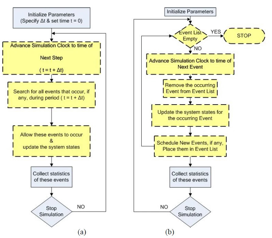
To understand the use cases and drawbacks of discrete-time simulation, let’s explore it more in-depth and compare it to its main alternative – discrete-event simulation (see Figure 1). DES is defined as
“a system designed to process some sort of entities with some kind of resources” (Choi, & Kang, 2013. p. 43).“During the simulated time between the occurrence of two successive events, the system state and entity attributes do not change in value. … the system state changes only when an event occurs” (Banks, et al., 2015, p. 130).
What is discrete-time simulation?

Discrete-time simulation, or DTS, is a type of simulation and a time advancement mechanism representing systems that change non-continuously over time. In simple words, DTS represents systems where state changes are only considered at specific points rather than continuously through time. Al Rowaei (2011, p. 250) defines DTS as:
“… a modeling paradigm in which the state variables change only at fixed time steps placed at a uniform rate. In DTS the system state variables can only be updated and changed at the fixed time steps (clock ticks). At every time-step (clock tick) at a uniform rate each state variable is checked for a possible update regardless of any event occurrence.”
Discrete-time simulation is an alternative to discrete-event simulation or DES. While both DTS and DES can simulate the same types of systems, they have significant differences that make them suitable for slightly different types of tasks.
In DTS, simulation time is divided into small, equal time intervals or step sizes. These steps have a fixed length that simulation engineers can sometimes set themselves. In literature, the length of the time interval in DTS is called delta t (Δt). For example, if the delta t is 2 seconds, the simulation will progress and record state changes every 2 seconds.
Discrete-time simulation vs discrete-event simulation
Earlier, we mentioned that discrete-time and discrete-event simulation could be used for the same tasks. Even if all simulation variables are tightly controlled, DES and DTS do not always converge to the same results (Buss and Al Rowaei, December, 2010).
We need to know how the two simulation approaches differ to understand why this can be the case. Without going into the details just yet, the differences between DTS and DES can be summarized as follows:
- In a DTS, simulation time progresses by a fixed amount that can often be selected by simulation engineers.
- In a DES, simulation time progresses every time changes occur in the system, e.g., when a customer enters or leaves a queue or when an agent reaches a waypoint.
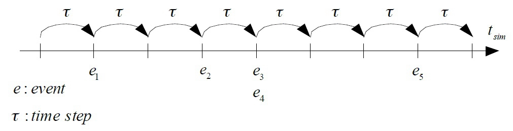
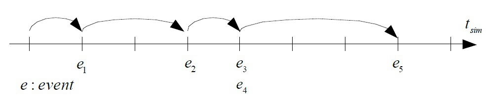
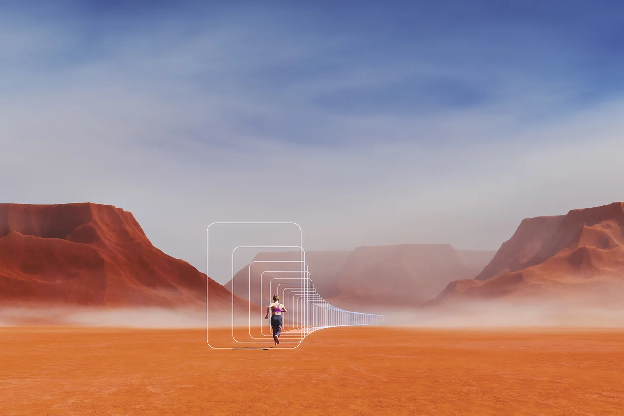
With this in mind, the time progression in DES is more dynamic and solely depends on the occurrence of events (see Figure 2), while DTS adopts a fixed approach that doesn’t depend on events (see Figure 3).
The differences between DTS and DES might be subtle, but they have enormous implications for the performance and outcomes of the two modeling approaches. One might expect that either method could achieve good results, but this isn’t the case.
The fact that DTS progresses time by some constant step size can dramatically affect the simulation results. Because some DTS packages don’t allow users to adjust step size, many engineers might not even be aware of the profound impact that it could have on simulation outcomes.
Research into the effect of step size on DTS outcomes is exceptionally scarce, and it’s unclear how exactly one can choose an optimal step size for their simulation needs. However, larger step sizes make simulation runs faster but less accurate. (Tang, et al., 2020). Let’s explore how below.
Step size and execution time
Let’s begin with the more intuitive aspect of the step size – its effect on the runtime of DTS models.
Generally, increasing the step size decreases the runtime of DTS models, while choosing smaller step sizes increase it. The reason is that with larger step sizes, the model doesn’t need to stop and update its state variables as frequently as with smaller step sizes. Essentially, large step sizes make the model skip larger chunks of time and do fewer calculations to update its state, which makes its execution faster.
Nevertheless, the number and spacing of events can significantly affect the runtime of both DES and DTS models. If the space between events is large, the DES model will be doing larger leaps from event to event, while DTS will keep progressing by its size even if no events occur between the steps. DES might be faster than DTS in cases like this, regardless of the step size.
But generally, unlike DES models, discrete-time simulations with larger step sizes can run much faster (Lucas and Armbruster, 2013). Because of this, if performance is a concern, then DTS models with large step sizes might be preferable. At least, this would be the case if the step size also didn’t affect simulation accuracy, which we’ll talk about next.
Step size and accuracy
The step size considerably affects simulation accuracy, meaning there’s a specific limit on how large simulation engineers should set their step sizes. The effect is so significant that it can nullify any performance advantage over DES gained by large step sizes.
While the mechanism behind step size vs. accuracy isn’t well understood, larger step sizes generally lead to poorer accuracy. In comparison, smaller step sizes can improve accuracy, bringing it closer to the accuracy of DES models.
The paper “A Comparison of the Accuracy of Discrete Event and Discrete Time” (Al Rowaei, et al., December, 2011) shared an interesting effect of increasing the step size in DTS. To investigate the impact of the step size on the accuracy of DTS, researchers ran two experiments, one of which involved an agent moving from point A to point B.
Researchers discovered that DTS performed very similarly to DES at tiny step sizes – the agent would reach point B as expected. However, increasing the step size at some point caused the agent to overshoot and oscillate around the target by some distance. The spread of overshooting increased with larger step sizes:
“We see that the agent must ‘backtrack’ to reach the target waypoint as the time step increases, although the agent will eventually reach the destination for time step sizes under a critical threshold. However, starting at a Δt of 1.3 seconds, the agent never stops at the target destination, instead oscillating back and forth between points on either side of the target waypoint forever” (Ibid., p. 2438).
Why did this happen? This effect may have been that large step sizes caused the DTS model to lose its granularity. When the model executed large steps, it may have lost critical information between the state transitions. This data loss could have prevented the model from adequately adjusting the agent’s state.
Another thing that the researchers observed was that the agent had to backtrack to reach its target. The simulation runtime increased roughly proportionately to the step size. The DES model performed the experiment much faster than the DTS model, regardless of step size. This impact demonstrated that larger step sizes didn’t necessarily reduce simulation runtime.
The paper also highlighted that when the system exhibited very high traffic, the DTS models showed poor accuracy even at tiny step sizes. If the state transitions were exceedingly frequent, the DTS models might fail to register them properly, leading to poor performance, regardless of the step size:
“We found no evidence of odd emergent agent behaviors using the DES methodology for any of the combat simulations studied. While the DES methodology may be less intuitive to simulation designers familiar with DTS environments, it is clear that the potential drawbacks from DTS are too great to use this method with combat simulations in decision-making contexts.In a complex simulation, the execution time of a DES model could possibly be slower than the corresponding DTS model with a large time-step Δt. While large time steps in a DTS model may execute faster than a corresponding DES model, our results here suggest that the outcomes of the DTS model could be seriously flawed. Perhaps more importantly, the modeler may be unaware that the model is producing erroneous results because of the size of the time step” (Ibid., p. 2440).
The disadvantages of DES compared to DTS
While DES might be more reliable than DTS, it has some disadvantages that can make researchers more inclined to use DTS models. Due to these disadvantages, DES isn’t as popular as DTS and isn’t as widespread in simulation software. Let’s take a look at these disadvantages below.
DES can be more difficult to implement than DTS
First, implementing DES models in code can be difficult because researchers need explicitly link state transitions to specific events. These events must be precomputed in advance to enable proper state transitions in the system. Event timing mechanisms also need to be implemented to enable the model to change its state at precisely the right time.
In contrast, in DTS, state transitions need to be connected to events. The mathematical expressions that define the system can be adapted to represent state transitions without explicit event lists. These formulae simplify the initial implementation of DTS models and make them more flexible because researchers can easily make changes to the simulation (Buss and Al Rowaei, December, 2010). Since there’s no need to manually link events to state changes, basically the adjustments to DTS models are applied “automatically.”
DES can sometimes be slower than DTS
While DES models are generally faster than DTS models while achieving comparable or better modeling accuracy, they can be slower in some instances. This particular case occurs if the system contains many events.
Because DES attends every single event in the system, it can slow down considerably if there are many interconnected events in the event list. DTS might not be affected by many events as much because it wouldn’t need to register every state change – it would just skip over some of the events because of its step size.
The disadvantages of DTS compared to DES
Now that we know the main disadvantages of DES, let’s look at the weaknesses of DTS. At a high level, the drawbacks of DTS boil down to the effect of the step size on speed and accuracy.
We’ve already looked at the effect of the step size on DTS – now, let’s discuss the implications of these effects.
The step size is an extra parameter that needs fine-tuning
The first problem with the step size is that it’s an additional parameter that simulation engineers might need to tweak to achieve reliable, accurate results in the DTS. Given the considerable effect of the step size on DTS output, choosing an optimal delta t is extremely important for the success of DTS models (Buss and Al Rowaei, December, 2010).
Unfortunately, not every DTS modeling package allows the user to adjust the step size, which is a significant problem. Step size that can’t be adjusted could drastically impact the results of the simulation without the engineers even knowing. Furthermore, a poorly selected step size could lead to researchers making wrong assumptions about their model.
To make matters worse, picking a reliable step size for DTS isn’t easy and requires experimentation. There are no precise guidelines or tips for step size selection because the impact of the step size can vary from model to model.
DTS step size might lead researchers to wrong conclusions
The second and much bigger issue with the step size is that it might lead researchers to the wrong conclusions about their simulation study.
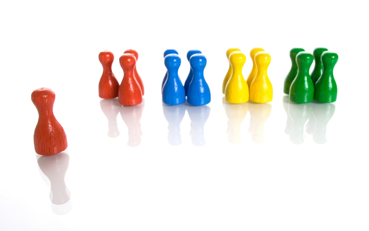
In the paper “A Comparison of the Accuracy of Discrete Event and Discrete Time,” (Buss and Al Rowaei, December, 2010) the researchers described an experiment where they had two color-coded combat agents with varying sensor ranges. The sensor range determined the distance the agent could spot and fire at the other agent. The sensor range was fixed at 30 meters for the blue agent and adjusted between 30 and 60 meters for the red agent. The adjustments for the red agent were made in 1-meter increments (see illustration in Figure 4).

The researchers discovered that when both agents had a sensor range of 30 meters, they had an equal chance of killing each other in both DES and DTS models. However, the results varied noticeably when the sensor range of the red agent increased even modestly.
In the DES model, every meter of added sensor range brought noticeable positive improvements in the kill rates of the red agent. In contrast, in the DTS model, the increase in the kill rates was less consistent and more erratic. The red agent in the DTS model saw improvement in its kill rates only every couple of meters, making progress more stepwise.
While it may have seemed that the models displayed the same general trend, they appeared to capture small details very differently. In this particular experiment, the DTS model failed to adequately represent the positive effect of the sensor range on kill rates. Overall, it did show that more range was better, but it had worse granularity than the DES model. The DES captured improvements with every change in the sensor range, whereas the DTS did not.
What are the implications of this disparity between DES and DTS? We can demonstrate them with a quick example.
Suppose a simulation team ran a similar experiment on a DTS model and did not experiment with a DES to double-check the results. Observing that increasing the sensor range did not bring consistent improvements to the red agent’s performance, the team could start investigating the reason for the stepwise changes, needlessly wasting time on reviewing results that weren’t even reliable. Furthermore, the simulation results could lead to engineers downplaying the effect of sensor range because of its inconsistent impact on kill rates.
Next steps
DTS has long been a viable choice for discrete simulation needs. It remains a powerful tool for simulation, but in view of the disadvantages we’ve explored in this article, some simulation teams might start leaning toward DES more. Both DTS and DES simulations can be modeled with a formal systems specification:
- Discrete Event System Specification [DEVS] (Zeigler, 2014).
- Discrete Time System Specification [DTTS] (Barros, 1997).
Both formalisms provide a language independent modeling specification for identifying specific event and time parameters and are useful for formally postulating a model before embarking upon the details associated with a specific simulation tool.
Even though DES can be more difficult to implement than DTS, its accuracy could be a significant advantage for many discrete simulations use cases. The benefits of DES could extend to fields like the military, medicine, healthcare, manufacturing, business, and even more niche areas like software delivery simulation. The Software Delivery Simulator leverages discrete-event simulation facilitating businesses to simulate software delivery pipelines efficiently and effectively.
Finally, simulation teams might need to weigh the benefits and drawbacks of DES and DTS to choose the right tool for their needs. However, in some situations, teams may be limited by the functionalities of the specific simulation software solutions available in their industries. Available simulation packages may not offer many choices to simulation teams. However, teams could consider building their simulation from scratch whenever this is the case. And once again, the team must decide between DES and DTS based on the pros/cons and implementation challenges.
With the inherent challenge of applying DTS and DES in the workplace, we would suggest a couple of inexpensive educational courses:
These seminars will help to get your feet wet.
References:
Al Rowaei, A. A. (2011). The Effect of Time-Advance Mechanism in Modeling and Simulation. Dissertation. Naval Postgraduate School.
Al Rowaei, A. A., Buss, A. H., & Lieberman, S. (2011, December). The effects of time advance mechanism on simple agent behaviors in combat simulations. In Proceedings of the 2011 Winter Simulation Conference (WSC) (pp. 2426-2437). IEEE.
Banks, J., Carson II, J. S., Nelson, B. L., & Nicol, D. M. (2015). Discrete-Event System Simulation. Pearson Education.
Barros, F. J. (1997). Modeling formalisms for dynamic structure systems. ACM Transactions on Modeling and Computer Simulation (TOMACS), 7(4), 501-515.
Buss, A., & Al Rowaei, A. (2010, December). A comparison of the accuracy of discrete event and discrete time. In Proceedings of the 2010 Winter Simulation Conference (pp. 1468-1477). IEEE.
Choi, B. K., & Kang, D. (2013). Modeling and Simulation of Discrete Event Systems. John Wiley & Sons.
Innocenti, E., Muzy, A., Aïello, A., Santucci, J-F. (2004). Parallel Discrete Event Simulation of Complex Propagation Phenomena: Parallel Interfaces and Cellular Environments. UMR CNRS 6134. U.F.R. Sciences et Techniques, University of Corsica.
Lucas, A., & Armbruster, B. (2013). Speeding Up Network Simulations Using Discrete Time. arXiv preprint arXiv:1302.5443.
Tang, J., Leu, G., & Abbass, H. A. (2020). Discrete time simulation. In Simulation and Computational Red Teaming for Problem Solving. IEEE, pp.143-155, doi: 10.1002/9781119527183.ch8.
Zeigler, B. P. (2014). Object-Oriented Simulation With Hierarchical, Modular Models: Intelligent Agents And Endomorphic Systems. Academic Press.