Introduction to continuous-time simulation
 April 2, 2022
 1143 words
 6 minutes to read

We’ve talked about discrete-event simulation [1] and agent-based simulation in previous posts. Now, we will have a look at continuous-time simulation – another important type of simulation modeling.
Continuous-time simulation is very distinct from other forms of simulation, and it has its own unique set of use cases. However, without understanding its capabilities and limitations, continuous-time simulation can easily be misused.
With that in mind, this post will explore the main features and use cases of continuous-time simulation! We’ll also compare continuous-time simulation with discrete-event simulation to give readers a better understanding of what it can and cannot do.
What is continuous-time simulation?
Continuous-time simulation is a type of simulation that continuously tracks the state of the target system. Differential equations often model systems in continuous-time simulation. These differential equations define how the state of the system changes over time.
Continuous-time simulations run on computers are rarely truly continuous-time simulations. Instead, digital computers perform continuous-time simulation approximately. There are two reasons for this:
- Real numbers cannot be represented faithfully because they are uncountable.
- Differential equations can only be solved approximately through some form of discretization.
Due to this, digital computers run continuous-time simulations by dividing (discretizing) time into small time steps, which is an approach called fixed-increment time progression. In some advanced cases, variable-increment time progression can be used.
Continuous-time vs discrete-event simulation – what’s the difference?
Discrete-event simulation is a significant alternative to continuous-time simulation, although many other types of simulation modeling exist.
At a high level, the primary differences between continuous-time and discrete-event simulations are listed in Table 1.
| Continuous-Time Models | Discrete-Event Models | |
|---|---|---|
| System Being Simulated | Specific mechanical unit with complex functioning | Multiple, often simple, entities |
| Definition of System State | Distribution of energy within system | Categorization of current system properties |
| Typial Measures of System State | Position, attitude, velocity (deterministic) | Queue size, incidence (statistical properties thereof) |
| Typical Factor Driving Updates | Time | Trasitions from state to state |
| Capability of Simulation | Analyze deterministic dynamic behavior of a mechanical unit | Analyze stochastic nature of interactions between entities |
| Common Uses | Design and analysis of unit, (real-time) training | Analysis and planning of operations with multiple entities |
In our introduction to discrete-event simulation, we’ve listed the following main characteristics of DES:
- Events occur at identifiable points in time.
- DES emphasizes events and state changes rather than the passage of time itself.
- DES uses time skipping – that is, it jumps between changes in the system, ignoring the state in between.
- DES often relies on queueing theory and uses different queueing systems to model a wide array of processes and phenomena.
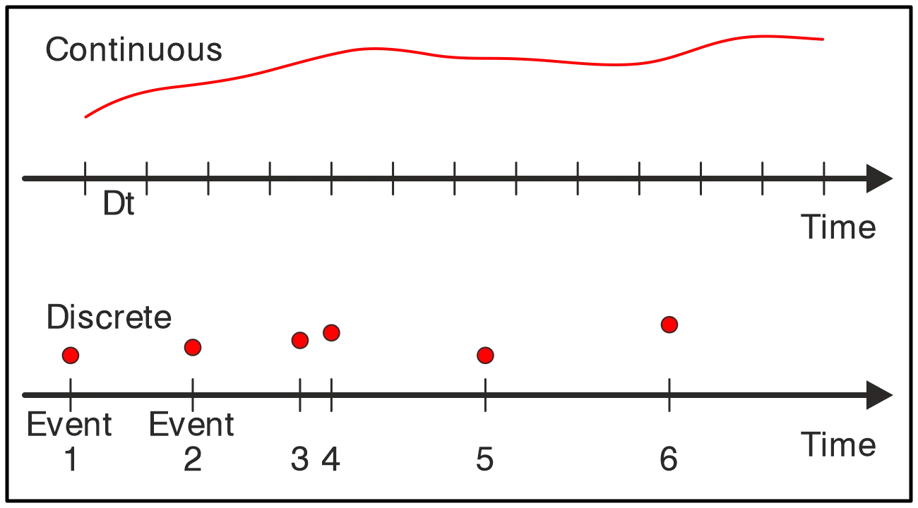
Continuous-time simulation directly contrasts these qualities. Specifically:
- Continuous-time simulation emphasizes the continuous change of the target system over time.
- Continuous-time simulation constantly tracks time and can produce data even when no changes occur in the target system.
- Continuous-time simulation is typically applied to natural sciences phenomena - like biological, chemical, and environmental processes. These applications are less likely to involve discrete queuing behaviors.
Because continuous-time simulation tracks system state continuously, it is more granular and, in certain situations (especially in the natural sciences), more accurate. On the other hand, continuous-time simulation can require more computational resources because continuous-time tracking of system states can be costly.
Another difference between continuous-time and discrete-event simulations is their adaptability to both continuous and discrete problems (Özgün and Barlas, 2009, July). More precisely:
- Continuous-time simulation can be used to model continuous and discrete processes. Although discrete processes are not continuous by nature, continuous-time models can successfully model them and generate valid results. However, a continuous-time model would require more time and computation for the same discrete problem. Additionally, for some discrete systems, the output of a continuous-time simulation model might not make sense.
- Discrete models could, in theory, be applied to continuous-time systems as well. However, a discrete-event model would provide a less refined insight into a continuous-time system because of its nature.
While there is some interoperability and encapsulation both ways, discrete-event simulation is particularly well-known for its ability to work with and encapsulate other simulations.
When to use continuous-time simulation?
Continuous-time simulation should be used to model systems that are expected to change continuously over time rather than at separate intervals. Some phenomena and processes that can be modeled with continuous-time simulation include:
- Cities,
- Climate,
- Ecosystems,
- Electric power and power grids,
- Flight dynamics,
- Hydraulics,
- Intelligent Complex Adaptive Systems,
- Temperature and humidity.
Continuous-time simulation can also be used to estimate the probability of different phenomena, like the probability of the breakdown of an industrial machine or the probability of a piece of programming code failing to meet quality requirements. Additionally, continuous-time simulation can be used in generative design or system control management tasks.
When NOT to use continuous-time simulation?
Continuous-time simulations are preferable with continuous phenomena and processes rather than discrete ones. Continuous-time simulation for discrete systems can be prohibitively time-/resource-consuming, although it can produce valid results.
Besides, the output of a continuous-time model for a discrete process might not always make sense. When a discrete output is expected (such as the integers 1 or 2), continuous-time models may generate results in between. Depending on the task, continuous outputs may not make sense and may even negatively affect the validity of a simulation.
Next steps
Continuous-time simulation can be useful in many situations. But more often than not, businesses will find that discrete-event simulation is more beneficial to their use cases. The ability of DES to efficiently model queues and process networks is instrumental when it is necessary to identify and fix bottlenecks in a system. Among other things, DES can be used to optimize queues, computer networks, manufacturing processes, or software delivery pipelines. A range of tutorials and descriptive articles are available at: SIM4EDU.COM.
Continuous-time simulation, in contrast, is better suited to simulating natural or physical phenomena. It’s also a good tool for simulating the probability of an event.
With all that in mind, as far as continuous-time and discrete-event models are concerned, there are no clear winners. Each method of simulation has its strengths and weaknesses (Fahrland, 1970). In order to choose the best simulation approach, businesses need to understand what they are trying to solve in the first place.
References:
Fahrland, D. A. (1970). Combined discrete event continuous systems simulation. Simulation, 14(2), 61-72.
Helal, M. (2008). A hybrid system dynamics-discrete event simulation approach to simulating the manufacturing enterprise. Doctoral Dissertation. University of Central Florida.
Özgün, O., & Barlas, Y. (2009, July). Discrete vs. continuous simulation: When does it matter. In Proceedings of the 27th International Conference of the System Dynamics Society (Vol. 6, pp. 1-22).
Pritchett, A. R., Lee, S. M., & Goldsman, D. (2001). Hybrid-system simulation for national airspace system safety analysis. Journal of Aircraft, 38(5), 835-840.