Input modeling as a foundation for simulation
 October 16, 2021
 2218 words
 11 minutes to read

Looking to start using simulation to optimize the enterprise’s business processes and enhance executive decision-making? If so, know that input modeling is one of the most important steps needed to set up the simulation project for success.
Input modeling is a complex process that requires a responsible and careful approach. The outcome of a simulation effort depends not only on the logic and structure of the modeling system but also on the quality of the input data. A discrete event simulation (DES) system is often founded upon stochastic probability elements. Specific probabilistic elements must be matched to the input model within a simulation system under investigation.
Remember the GIGO (garbage in, garbage out) concept whenever defining the inputs is attempted – the model will only be as good as the data fed into it.
To whet the team’s appetite, this taxonomy proposes a wide range of input models (see Figure 1):
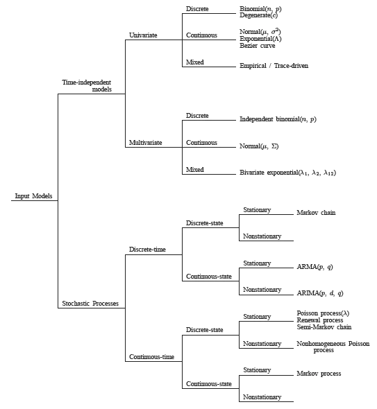
With that, we propose a quick-start guide for input modeling to help to formulate a sound simulation plan! We won’t be delving into the mathematical aspects of input modeling too much – tools exist that can take care of the computations. We will also not be covering every type of input model as outlined by Leemis above. Rather, our goal is to introduce the steps and challenges of input modeling in an easy-to-grasp manner, including:
- How can useful data for the model be identified?
- Which probability distributions should be adopted for input modeling?
- How are parameters estimated for candidate probability distributions?
- How is the goodness of fit of candidate probability distributions determined?
What is input modeling in simulation?
To get started, what is input modeling, and why is it important? Currently, the simulation of real-world processes with 100% accuracy is either impossible or extremely challenging. This is due to uncertainty – even if we possess a good understanding of a process, we often don’t have full information about the variables that can impact it.
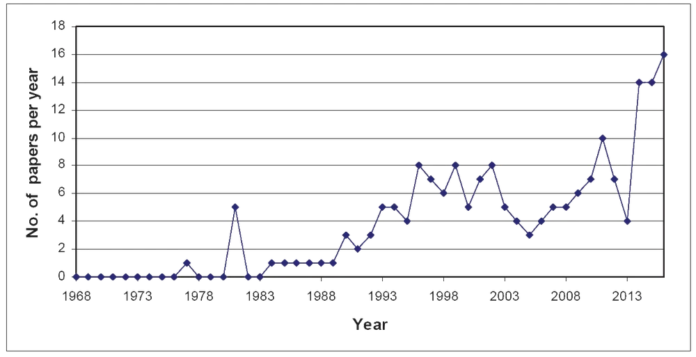
Input modeling in simulation has increased in importance, as demonstrated by the growing number of academic articles published by the Winter Simulation Conference Proceedings over the last 50 years (see Figure 2), especially with the advent of high-performance computer-based simulation.
Input modeling in simulation aims to help manage uncertainty in data and come up with approximations that represent a system with sufficient accuracy. Modeling of inputs relies on probability distributions. If the data distribution can be well approximated, a model can likely be identified. Quality inputs facilitate the construction of a simulation that produces valid results. Based on these results, business processes can be optimized.
The four phases of input modeling for simulation
To come up with high-quality inputs for the enterprise’s simulation needs, a structured approach to input modeling should be adopted. As a general rule, input modeling is broken down into the following four phases:
- Data collection.
- Identification of the input data distribution.
- Parameter estimation for the selected distribution.
- Estimation of the goodness of fit.
The process of input modeling may seem quite simple on the surface. To ensure that erroneous assumptions about input data are not being made, various details need to be kept in mind. To help keep input modeling on the right track, let’s now have a look at each of the listed four steps!
Step 1 – Data collection

The quality of the data obtained from the system under investigation is paramount to accurate input modeling. Ideally, huge amounts of data will be acquired to provide a useful representation of the target system.
Depending on the process and the toolset available, a large collection of data may not be feasible. While following the “the more, the better” philosophy can simulate input modeling with better accuracy, the thousands or hundreds of thousands of data points are not necessary to get started. Input modeling would be possible even if no data was available, though the model’s initial quality would be comparatively low until more samples are gathered.
Regardless, with data collection, make sure to remember the following points:
- Data collection is based on observation. To commence input modeling, the simulation environment should be monitored, and relevant data points collected. This will take time, so data should be gathered as soon as possible.
- Data needs to be representative of the process being modeled. Any old data should not be collected – rather, data should be collected that is relevant and valid for the goals of the simulation. Although more data is always great, useless information shouldn’t be collected for the sake of having more to feed into the model.
- Data should be collected over a continuous time period. Observations must cover a continuous timeframe. Gaps in data may conceal crucial temporal relationships between data points and may lead to wrong conclusions about the data distribution.
- Variables may be related or dependent on each other. For simplicity, variables in data are often considered to be independent of each other. With some processes, the assumption of independence won’t hurt, but if the data contains any significant interdependencies, those interdependencies need to be demonstrated during analysis. Using scatter plots is one way of checking variables for dependence.
Step 2 – Identification of the input data distribution
Once sufficient data has been collected, a probability distribution to represent the data needs to be adequately demonstrated.
How is the distribution of the data described? Well, five primary factors that decide the choice of distribution are:
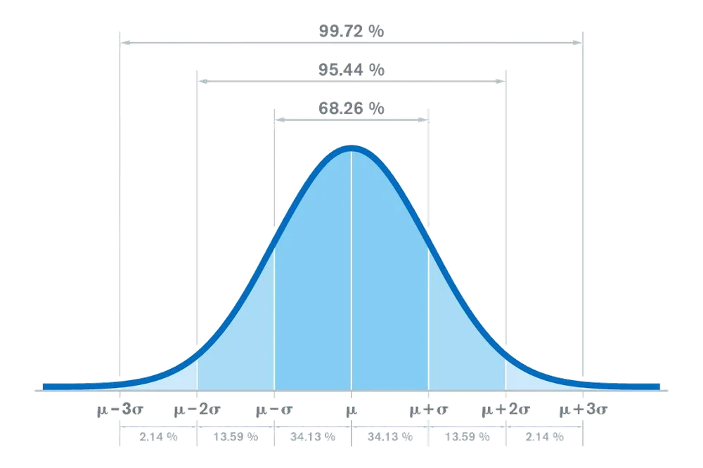
- The shape of the data’s histogram. Graphically demonstrating the frequency (or count) of values in a dataset, histograms are an excellent method for evaluating the shape of the data distribution. In many cases, histograms point to the right probability distribution by just their appearance. For example, if a data histogram resembled a bell, the optimal distribution would probably be the normal distribution.
- The context and intended use of the data. Aside from the histogram, the context and intended use of the data should be considered. For example, the exponential distribution would probably be adopted if the time until some event needs to be estimated – such as the arrival of a customer or breakdown of a machine. Or, if the number of events occurring in some time frames was estimated, the Poisson distribution might be chosen.
- Whether correlation or dependency exists between variables. As mentioned earlier, variables are typically assumed to be independent of each other to simplify distribution selection. This assumption may sometimes lead to poor simulation results, forcing the use of more complex distributions that can represent autocorrelative processes, time-series data, or multivariate inputs.
- Whether the process changes over time. Standard distributions often assume that the data distribution along with its parameters stays fixed over time. Unfortunately, this isn’t always the case, which complicates input modeling. If the target process changes over time, a flexible input model could be chosen (such as the Pearson or Johnson systems), or approximate parameters over some short time period could be chosen, adjusting the model as the system changes.
- The interval (range) of the data. A certain range of values also binds many probability distributions (e.g., only positive or constrained between certain values a and b). To ensure that the model doesn’t produce nonsensical results and comprehensively covers the data, the range of candidate distributions (or, mathematically speaking, the support) needs to be checked.
To keep the distribution selection process “compliant” with these five points, data should be abundant.
With that said, useful distributions exist for cases where there is very little data about the target process. For example, if only the minimum and maximum values to describe the process occur, the uniform distribution would be the starting point. If the most likely value is known, a switch could be initiated to the triangular distribution for slightly more accurate modeling. Distributions like these will not be highly accurate, but they will provide some foothold for analysis.
We have a separate post detailing some of the most important probability distributions – it could provide additional background information for distribution selection.
Step 3 – Parameter estimation for the selected distribution
The next step would be to estimate the values of the parameters required by the selected probability distribution. Probability distributions are defined by certain parameters, which is why sufficiently accurate values need to be obtained.
Here are a few examples of probability distributions and their parameters:
- Normal distribution – mean and variance/standard deviation.
- Poisson distribution – average arrival rate over the observed timeframe.
- Bernoulli distribution – the probability of success/failure in a yes-no (binary) experiment.
- Continuous uniform distribution – lower and upper bounds of the input values.
- Triangular distribution – lower and upper bounds of the input values and the most likely value (the mode, in other words).
A common method of parameter estimation is maximum likelihood estimation (MLE). With MLE, a set of parameters can be proposed that allows the selected distribution to match the real data as closely as possible. In the language of statistics, MLE implies the selection of parameters that maximize the probabilities of the observed data in the chosen model.
Another popular method is least-squares estimation, where parameters are picked to minimize the discrepancies between the observed data and the model’s output – just like with MLE. However, from a mathematical standpoint, the least-squares method minimizes the differences between target and predicted values.
Other methods of parameter estimation include the method of matching moments and the method of matching percentiles.
In cases where no data is available to perform parameter estimation, other possible data sources could be utilized:
- Expert opinion. Experts in the industry may provide educated and reasonable guesses about the process, including minimum and maximum values, most frequent values, and variance.
- Engineering data. If the process has spec sheets, performance data, and other similar documents, they could be used for effective input modeling.
- Physical limitations. Some parameters may be obtained for the model by reviewing the physical limitations of the process. At the very least, this may allow the determination of lower and upper bounds for the parameters and may also result in an educated guess about the data’s mean and standard deviation/variance.
Step 4 – Estimation of the goodness of fit
Goodness of fit tests estimate the closeness between the real data and the samples that the selected probability distribution produces. Many methods for estimating goodness of fit exist – some popular ones are:
- Kolmogorov-Smirnov test.
- Anderson-Darling test.
- Chi-Square test.
- Probability plots.
- Density-histogram plots.
Note that these tests emphasize different areas in the data. For example, the Kolmogorov-Smirnov test weights the importance of discrepancies in the middle of the data, while the Anderson-Darling test accentuates discrepancies in the tails.
Additionally, keep in mind that tests for goodness of fit only numerically demonstrate the degree of fit since they result in a number. Such a number may be useful, but it doesn’t explain where discrepancies have occurred. Fortunately, plots facilitate visually checking the quality of fit.
Regardless, no single correct test for the estimation of goodness of fit exists. For the best results, several tests should be executed to better understand how the selected probability distribution performs.
Two other important points to remember with goodness of fit tests:
- If little data exists, any distribution could show good results.
- If plenty of data exists, no distribution may show good results.
Therefore, goodness of fit tests should be undertaken with a grain of salt – they are beneficial, but their results can be misleading. If the distribution of the target data has been estimated reasonably well, but poor scores are encountered, then the model’s output should be checked to determine if it makes sense and meets expectations (as should be done for simulation validation).
Next steps
The team does not have to include mathematics gurus to choose an adequate distribution for input modeling. True, a good degree of understanding of the data and the process of the simulation is necessary. However, many tools are available to carry out heavy lifting (i.e., calculations).
Modern simulation packages and platforms often support the input modeling process, offering tips for distribution selection and facilitating the performance of goodness of fit tests. Programming languages like Python or R also allow the completion of statistical tests to help estimate parameters and check for fit quality.
We encourage the team members to familiarize themselves with the different methods of input modeling for further simulation. But remember, understanding all the ins and outs is unnecessary!
References:
Biller, B., & Gunes, C. (2010, December). Introduction to simulation input modeling. In B. Johansson, S. Jain, J. Montoya-Torres, J. Hugan, E. Yücesan, R. Pasupathy, R. Szechtman, and E. Yücesan, Proceedings of the 2010 Winter Simulation Conference (pp. 49-58). IEEE.
Cheng, R. (2017, December). History of input modeling. In W. K. V. Chan, A. D’Ambrogio, G. Zacharewicz, N. Mustafee, G. Wainer, and E. Page, (Eds.), 2017 Winter Simulation Conference (WSC) (pp. 181-201). IEEE.
Leemis, L. (1999, December). Simulation input modeling. In D.J. Medeiros, E.F. Watson, J.S. Carson, and M.S. Manivannan, (Eds.), Proceedings of the 31st Conference on Winter Simulation: Simulation—a Bridge to the Future-Volume 1 (pp. 14-23).
Günes, M. Spaniol, O. (2007, April 20). Course: Simulation - Modeling and Performance Analysis with Discrete-Event Simulation. Presentation Slides, Chapter 9. Freie Universität Berlin. (http://www.nets.rwth-aachen.de/content/teaching/lectures/sub/simulation/simulationSS07/)