A gentle introduction to discrete-event simulation
 March 12, 2022
 1444 words
 7 minutes to read

Simulation is a many-sided beast, and research teams should approach it with extra care. There is no single simulation approach or tool suitable for all tasks – teams need to identify their research goals and choose a method accordingly.
Discrete-event simulation is just one of the options available to businesses and researchers. Like any other simulation method, it can be highly effective in certain situations and virtually useless in others. However, despite its relative conceptual simplicity, discrete-event simulation can be a powerful tool in the right hands.
What is discrete-event simulation?
Discrete-event simulation, or DES, is intended to simulate systems where events occur at specific, separable instances in time. DES contrasts with a continuous simulation where events are tracked continuously.
DES can be either deterministic or stochastic, depending on the nature of the target process. The defining characteristics of discrete-event simulation are as follows:
- Events occurring at specific points in time. As mentioned earlier, DES is used to model processes or systems that change at identifiable time instances. DES does not track system state continuously.
- Emphasis on events. Changes in state and events are the focus of DES, hence why DES is often referred to as “event-driven.”
- Time skipping (next-event time advance). Typically, DES does not consider the system’s state between events, instead “jumping” to subsequent events as the simulation progresses. Time skipping reduces the complexity and resource intensity of discrete-event simulations.
- Heavy use of queueing theory. Queueing theory is the cornerstone of many discrete-event simulations, defining how resource-constrained processing is executed. Although queueing theory is not always used in DES, it can be used whenever the arrival and the service of requests are the features of interest.
Thus, simply put, DES could be defined as “a system designed to process some sort of entities with some kind of resources” (Choi, & Kang, 2013. p. 43).
A contrast and compare of DES with continuous simulation would yield the characteristics outlined in Table 1.
| Discrete-Event Simulation | Continuous Simulation | |
|---|---|---|
| Changes in the target system | No changes occur between events | The system changes continuously with the passage of time |
| Primary characteristic | Events are the primary characteristic of discrete-event simulation | Time is the primary characteristic of continuous simulation |
| Time tracking | Models “jump” from event to event in time because the state between events is irrelevant | Models track the system continuously over time |
The attributes of discrete-event simulation
At a high-level, discrete-event simulation is built on top of the following components:
- System – a collection of entities with certain attributes.
- State – a collection of attributes representing the system’s entities.
- Event – an occurrence in time that may alter the system’s state.
On a more technical level, discrete-event simulation has the following components (Law & Kelton, 2007, p. 10-11):
- System state – a collection of variables that represent the state of the simulated system.
- Simulation clock – a variable that tracks the passage of time in the simulated system.
- Event list – a collection of when each type of event will occur.
- Statistical counters – variables that contain statistical information about the system, such as average request processing time, server load, or average queue length.
- Initialization routine – the routine that defines how the model selects the first event at time 0.
- Timing routine – the routine that selects the next event from the event list and jumps in time to its execution.
- Report generator – the routine that defines how the program calculates and updates statistical counters and includes them in a post-run report.
- Event routine – a routine that updates the system’s state when a particular type of event occurs.
- Library routines – routines that use probability distributions to generate random values for uncertain variables in the system.
- Main program – a program that invokes the model’s routines to perform the simulation.
The process of discrete-event simulation
Such a breakdown of components allows for a greater degree of adjustability in discrete-event simulation. Simulation engineers can easily fine-tune how the program initializes the simulation, selects events, progresses time, and reports results.
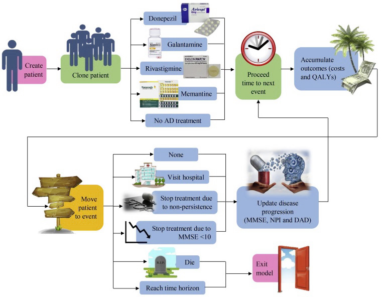
Figure 1 depicts the process encompassing the discrete-event simulation.
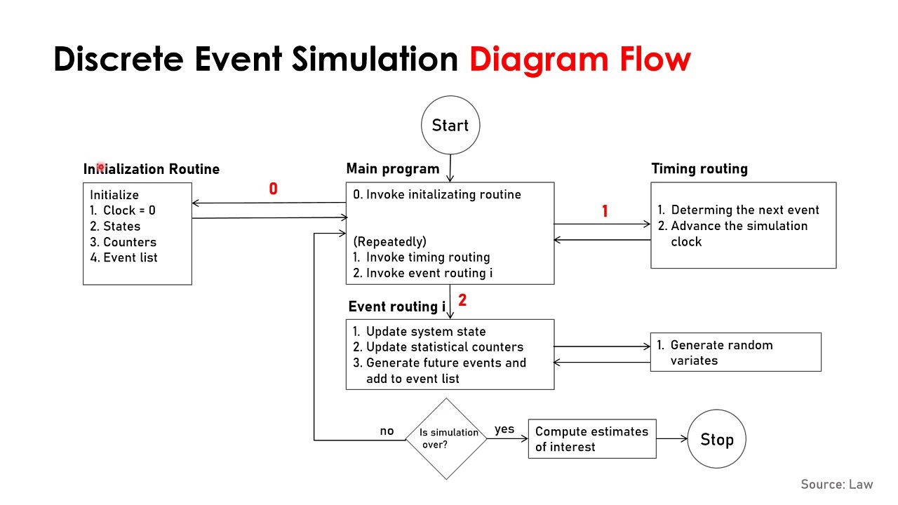
This processing aims to check for bottlenecks, find blocked or starved locations, operations, or sources, identify failure modes, and improve the design. Some examples of probability distributions are highlighted in Figures 2 and 3.


When to use discrete-event simulation
To give readers a better idea of the uses of discrete-event simulation, here are a few situations or problems that DES can help businesses solve:
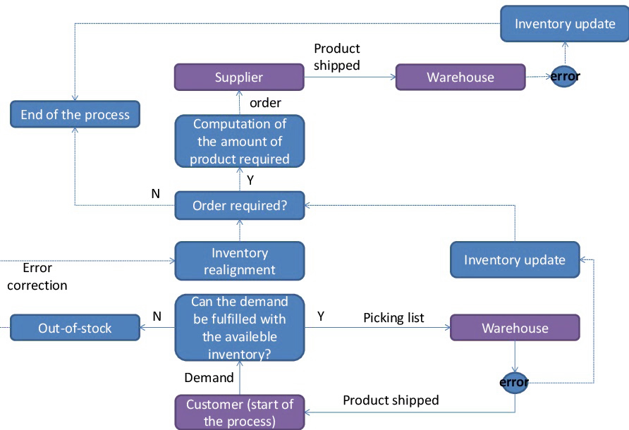
- Inventory management. Discrete-event simulation can be used to estimate how much inventory is necessary to, on the one hand, satisfy existing demand and, on the other hand, minimize the waste of space and labor (Figure 4).
- Queue optimization. DES can be beneficial in optimizing queues, like queues in a bank, health care facility, or a customer support center. With queues, metrics like the frequency of new request arrival, duration of request processing, and the number of servers allow businesses to assess the performance of their systems and make adjustments to them as necessary (Figure 5).
- Optimization of computer networks. Like queue optimization at physical locations (such as a bank), DES may be used to fine-tune computer networks. Discrete-event simulation can specifically help businesses assess their network capacity vs. demand, estimate bandwidth, and identify bottlenecks (Figure 6).

To summarize these examples, discrete-event simulation is optimal for the following situations:
- When the team wants to describe processes where changes occur instantaneously, at particular points in time.
- When the quantity of interest (like inventory or software installations) is countable.
When NOT to use discrete-event simulation
Discrete-event simulation is suboptimal for modeling systems that change continuously. However, it can represent continuously valued phenomena and can even produce sensible results. Still, DES provides comparatively low definition and accuracy when applied to continuous systems.
Continuous simulation can help us track how a process develops over time, capturing its state at many points without any gaps or jumps. Discrete-event simulation, albeit capable of producing valid results with continuous systems, may not accurately represent continuous phenomena since it only tracks time events at discrete points.
With that in mind, DES is best to use with discrete systems, though it can theoretically be used with continuous systems when it is necessary to obtain insights quickly.
Next steps
Although discrete-event simulation is just one among many simulation modeling methods, it is helpful in a vast range of situations. However, it is not always the best tool for the job. Any easy way to become acquainted with discrete-event simulation is an introductory Discrete Event System Simulation course through Udemy. Another approach to learning about DES is to review a well-developed engineering teaching case: The Skateboard Factory (Mesquita, et al., 2017).
When choosing an approach to simulation, it is essential to understand what the team is trying to simulate. More concretely, the team should have a statistical knowledge of the target system – whether it is continuous or discrete, deterministic or stochastic, or static or dynamic.
Apart from choosing the right simulation approach, businesses should also determine if a simulation is the right solution to their issues in the first place. Although a powerful tool, simulation can be overkill in situations where the system state can be predicted easily and reliably.
References:
Bottani, E., Mantovani, M., Montanari, R., & Vignali, G. (2017). Inventory management in the presence of inventory inaccuracies: an economic analysis by discrete-event simulation. International Journal of Supply Chain and Inventory Management, 2(1), 39-73.
Choi, B. K., & Kang, D. (2013). Modeling and simulation of discrete event systems. John Wiley & Sons.
Harahap, E., Nurrahman, A., & Darmawan, D. (2017). A modeling approach for event-based networking design using MATLAB-SimEvents. Proceedings of 2nd International Multidisciplinary Conference 2016, Jakarta, Indonesia, 1(1). 327-331
Kongpakwattana, K., & Chaiyakunapruk, N. (2020). Application of discrete-event simulation in health technology assessment: a cost-effectiveness analysis of Alzheimer’s disease treatment using real-world evidence in Thailand. Value in Health, 23(6), 710-718.
Law, A. M., Kelton, W. D. (2007). Simulation modeling and analysis (3rd ed.). New York: McGraw-Hill.
Mesquita, M. A., Mariz, F. B. A. R., & Tomotani, J. V. (2017). The Skateboard Factory: a teaching case on discrete-event simulation. Production, 27(spe), e20162262. http://dx.doi.org/10.1590/0103-6513.226216